In this tutorial, we’ll explore Generalized Policy Iteration (GPI) through two approaches:
- SARSA (model-free) – Learns directly from experience without knowing the environment’s transition dynamics.
- Policy Iteration (model-based) – Uses a known transition model to compute an optimal policy.
We’ll implement both on FrozenLake-v1 (deterministic) and compare their learning behaviors.
1. Understanding Generalized Policy Iteration (GPI)
GPI consists of two key alternating steps:
- Policy Evaluation: Estimate the action-value function $ Q^\pi(s, a) $ for a given policy $ \pi $.
- Policy Improvement: Use $ Q^\pi(s, a) $ to derive a better policy $ \pi’ $.
This iterative process continues until convergence. SARSA learns purely from interaction, whereas Policy Iteration exploits the known dynamics.
We’ll use deterministic Frozen Lake:
- State space: $ 4 \times 4 = 16 $ discrete states.
- Action space: $ {0: \text{left}, 1: \text{down}, 2: \text{right}, 3: \text{up} } $.
- Rewards:
- $+1$ if reaching goal.
- $0$ otherwise.
- Stepping into a hole ends the episode.
State Transition Table
For example, in the initial state ($s=0$):
- Action Right (2) → Moves to $s=1$.
- Action Down (1) → Moves to $s=4$.
- Actions Left (0), Up (3) → No effect (remains in $s=0$).
We’ll now implement both SARSA (model-free) and Policy Iteration (model-based).
3. SARSA (Model-Free)
SARSA learns from experience without knowledge of the transition model. The algorithm updates the Q-function using the following temporal difference (TD) learning rule:
\[Q(s_t, a_t) \leftarrow Q(s_t, a_t) + \alpha \left( r_t + \gamma Q(s_{t+1}, a_{t+1}) - Q(s_t, a_t) \right)\]where:
- $ Q(s_t, a_t) $ is the action-value function at state $ s_t $ and action $ a_t $.
- $ \alpha $ is the learning rate.
- $ r_t $ is the immediate reward received after taking action $ a_t $.
- $ \gamma $ is the discount factor.
- $ Q(s_{t+1}, a_{t+1}) $ is the action-value estimate for the next state-action pair.
We can rewrite the SARSA update using the expected value operator to better understand its theoretical meaning.
\[Q(s_t, a_t) = \mathbb{E} \left[ r_t + \gamma Q(s_{t+1}, a_{t+1}) \mid s_t, a_t \right]\]Expanding it using the law of total expectation:
\[Q(s_t, a_t) = \sum_{s'} P(s' | s_t, a_t) \sum_{a'} \pi(a' | s') \left[ R(s_t, a_t) + \gamma Q(s', a') \right]\]and we can use it to update the Q-function iteratively, as in the code below, according to the expected transition probabilities, rather than the actual knowledge of true transitions from some environment model. Additionally, note that SARSA is an on-policy method, meaning it approximates the value function using observations gathered through the policy it is currently following and updating.
class SARSAAgent:
    def __init__(self, state_size, action_size, alpha=0.1, gamma=0.99, epsilon=0.1):
        self.state_size = state_size
        self.action_size = action_size
        self.alpha = alpha
        self.gamma = gamma
        self.epsilon = epsilon
        self.q_table = np.zeros((state_size, action_size))

    def choose_action(self, state):
        if np.random.rand() < self.epsilon:
            return np.random.choice(self.action_size)  # Explore
        return np.argmax(self.q_table[state])  # Exploit

    def update(self, state, action, reward, next_state, next_action):
        td_target = reward + self.gamma * self.q_table[next_state, next_action]
        if not terminated:
            td_target += self.gamma * self.q_table[next_state, next_action]

        td_error = td_target - self.q_table[state, action]
        self.q_table[state, action] += self.alpha * td_error

    def decay_epsilon(self):
        self.epsilon = max(0.01, self.epsilon * self.epsilon_decay)
def train_sarsa(env, agent, episodes=500):
    rewards_per_episode = []

    for episode in range(episodes):
        state, _ = env.reset()
        action = agent.choose_action(state)
        total_reward = 0

        while True:
            next_state, reward, terminated, truncated, _ = env.step(action)
            next_action = agent.choose_action(next_state) if not terminated else 0
            agent.update(state, action, reward, next_state, next_action)

            state, action = next_state, next_action
            total_reward += reward

            if terminated or truncated:
                break

        agent.decay_epsilon()
        rewards_per_episode.append(total_reward)

    return rewards_per_episode
4. Policy Iteration (Model-Based) Implementation
Since we know the true transition model, we can compute the optimal policy iteratively using the Bellman equations. The main takeaway is that Policy Iteration explicitly computes the expectation over all transitions using the true transition probabilities instead of sampled transitions, which is the main difference from SARSA.
4.1 Policy Evaluation
We estimate $ V^\pi(s) $ using the Bellman equation:
\[V^\pi(s) = \sum_a \pi(a|s) \sum_{s'} P(s' | s, a) [R(s, a) + \gamma V^\pi(s')]\]def policy_evaluation(policy, env, gamma=0.99, theta=1e-6):
env = env.unwrapped
V = np.zeros(env.observation_space.n)
while True:
delta = 0
for s in range(env.observation_space.n):
v = V[s]
V[s] = sum(policy[s, a] * sum(
p * (r + gamma * V[s_]) for p, s_, r, _ in env.P[s][a]
) for a in range(env.action_space.n))
delta = max(delta, abs(v - V[s]))
if delta < theta:
break
return V
4.2 Policy Improvement
Then, we update the policy using the Bellman optimality equation:
\[\pi(s) = \arg\max_a \sum_{s'} P(s' | s, a) [R(s, a) + \gamma V^\pi(s')]\]In both the policy evaluation and improvement steps, we use the true transition probabilities $ P(s’ | s, a) $ to compute the expected value over all possible transitions. If either we do not have access to the true transition probabilities or make no assumptions of the underlying environment when calculating the expected value, we resort to model-free methods like SARSA. Additionally, given the model, the Policy Iteration step can calculate the optimal policy directly through iterative computation, without requiring interaction with the environment.
def policy_improvement(V, env, gamma=0.99):
    env = env.unwrapped
    policy = np.zeros((env.observation_space.n, env.action_space.n))

    for s in range(env.observation_space.n):
        q_values = np.zeros(env.action_space.n)
        for a in range(env.action_space.n):
            q_values[a] = sum(p * (r + gamma * V[s_]) for p, s_, r, _ in env.P[s][a])
        best_action = np.argmax(q_values)
        policy[s] = np.eye(env.action_space.n)[best_action]  # One-hot encoding

    return policy
4.3 Policy Iteration Algorithm
def policy_iteration(env, gamma=0.99):
    policy = np.ones((env.observation_space.n, env.action_space.n)) / env.action_space.n

    while True:
        V = policy_evaluation(policy, env, gamma)
        new_policy = policy_improvement(V, env, gamma)

        if np.array_equal(new_policy, policy):
            break
        policy = new_policy

    return policy, V
5. Running on FrozenLake-v1
env = gym.make("FrozenLake-v1", is_slippery=False, render_mode=None)

agent = SARSAAgent(state_size=env.observation_space.n, action_size=env.action_space.n, alpha=0.1, gamma=0.99,
                   epsilon=0.1)

sarsa_rewards = train_sarsa(env, agent, episodes=int(1e3))
sarsa_rewards = np.convolve(sarsa_rewards, np.ones((100,)) / 100, mode='valid')

policy, V = policy_iteration(env, gamma=0.999)
plt.plot(sarsa_rewards, label="SARSA")
plt.axhline(V[0], color='r', linestyle='--', label="Optimal Value from Model-Based")
plt.xlabel("Episodes")
plt.ylabel("Total Reward")
plt.title("SARSA vs. Policy Iteration Performance")
plt.legend()
plt.show()
And we can observe the learning behaviors of SARSA and Policy Iteration on FrozenLake-v1.
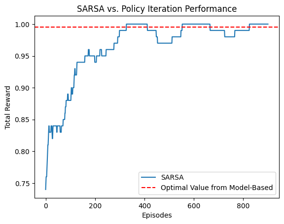
Noticeably the model-based Policy Iteration results in a near perfect policy (with a reward of 1 in all episodes), while the SARSA model-free method learns more slowly and fluctuates in performance.
We can summarize the key differences between SARSA (model-free) and Policy Iteration (model-based) as follows:
| Feature | Model-Free (SARSA) | Model-Based (Policy Iteration) |
|---|---|---|
| Requires transition probabilities? | No | Yes |
| Exploration needed? | Yes | No (if model is exact) |
| Convergence speed | Slow (data-dependent) | Fast (if model is correct) |
| Robust to model errors? | Yes | No |
| Computes | $ Q(s, a) $ using Sampled transitions | Full expectation over transitions |
| Requires $ P(s’ s, a) $? | No | Yes |
- SARSA (Model-Free) learns slowly but does not require transition knowledge.
- Policy Iteration (Model-Based) finds the optimal policy immediately but assumes perfect knowledge.
- Trade-off: SARSA is more adaptable to real-world settings, while policy iteration is efficient for known environments.